If you take any pure $N$-qubit product state
and evolve it with arbitrary 2-body Hamiltonian
the initial evolution of the sector lengths $A_k$ of the evolved state $\ket{\phi_t} = \exp(-iHt)\ket\phi$ will take the following form
Crucially, (a) the value at $t=0$ is the same for all product states due to LU-invariance of $A_K$, (b) first time derivative vanishes, and (c) second time derivative has the same overall structure with binomial coefficients for any initial product state and Hamiltonian weights (modulo the prefactor – naturally, if you have larger weights, the derivative is larger).
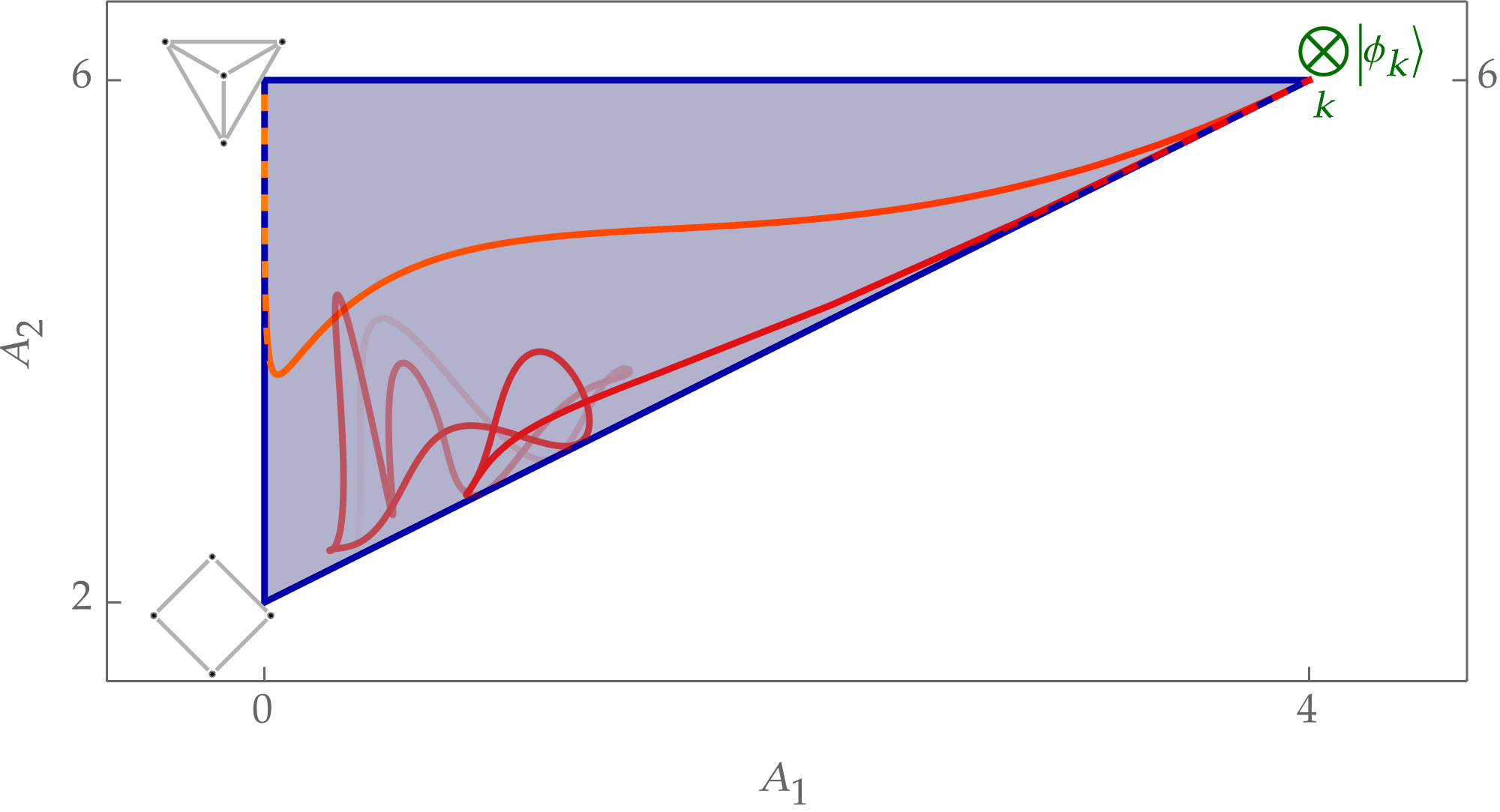
In the following image the evolution of two 4-qubit states is superimposed on the triangle of all allowed $(A_1, A_2)$ sector lengths of pure states. The left triangle corners are denoted with graphs corresponding to the graph states: top left is the GHZ state, bottom left is the state $\text{CZ}_{12} \text{CZ}_{23} \text{CZ}_{34} \text{CZ}_{41} \ket{+}^{\otimes 4}$, while product states lie at the right corner. Orange curve corresponds to a precisely selected Ising-like Hamiltonian leading to the GHZ state formation; red line is a random Hamiltonian and random initial product state. Observe that their initial slope in the right part of the picture is the same!
Simplifications and preliminary info
Since sector lengths are local unitary invariant, we can rotate each qubit to $\ket\uparrow$ without loss of generality. On this state only products of $\sigma^z$ and identity have nonzero expectation values (with all expectation values of this form equal to 1).
Furthermore, recall that single-qubit Paulis either commute (if they are equal, $[\sigma^z,\sigma^z]=0$ – sorry for stating the obvious but it helps later) or anticommute. For two Pauli strings $P$ and $Q$ the commutator $[P,Q]$ vanishes iff the number of anticommuting sites is even. Crucially: they also either commute, or anticommute! So, if the number of anticommuting sites is odd, $PQ+QP=0$.
First derivative vanishes
We have
and on the all-$\ket{\uparrow}$ state, $\langle P \rangle$ is nonzero (and equal to 1) only if $P$ is a $z$-string. Concentrate on a single Hamiltonian term $h_{ij}^{ab} \sigma_i^a\sigma_j^b$. For $[P,\sigma_i^a\sigma_j^b]$ to be nonzero (as an operator, before expectation value calculation), the two strings must anticommute, meaning only one $i$ or $j$ must carry either $\sigma^x$ or $\sigma^y$ at a position where $P$ has $\sigma^z$. But then the resulting product has a non-$z$ Pauli at this site, so it all vanishes: if $\langle P\rangle\neq 0$, $\langle [P,\sigma^a_i\sigma^b_j]\rangle =0$.
All the terms vanish, so $\partial_t A_K=0$ for all $K$. Let's see the behavior of the second time derivative.
Second derivative doesn't but it's a bit complex
The first time derivative happened to vanish all the time, we look at the second. Product rule gives
At $t=0$ on the $\ket{\uparrow}^N$ state, the two terms have disjoint support: first term is nonzero only for non-$z$-strings (this is just a necessary condition and not full characterization), as we just showed $\partial_t \langle P\rangle =0$ for $z$-strings; second is nonzero only for $z$-strings because of the $\langle P\rangle$ prefactor. Both are quadratic in $h_{ij}^{ab}$, and our aim will be to build a bilinear form capturing the terms. We treat the two terms (first time derivative squared, and second time derivative) separately and will combine them later.
The $\langle P\rangle \partial_t^2 \langle P\rangle$ term
For a $z$-string $P$ with $K$ sites containing $\sigma^z$, the second term gives (at $t=0$):
Expanding $H$ twice, we get a sum of double commutators $[[\sigma_i^a\sigma_j^b, P], \sigma_k^c\sigma_l^d]$. For the expectation on the all-up state to survive, the result must be a $z$-string.
But first $P$ must survive the inner commutator: by the same parity argument as before exactly one site in ${i,j}$ must anticommute with $P$, flipping exactly one $\sigma^z$ of $P$ to a $\sigma^x$ or $\sigma^y$ (otherwise the entire commutator is zero). Outer commutator must then turn the entire expression into a $z$-string, and this requires that both Hamiltonian terms $h^{ab}_{ij}$ and $h^{cd}_{kl}$ act on the same edge ($(i,j)=(k,l)$), as otherwise surviving non-$z$ Paulis vanish th expectation value. The two commutations produce a bilinear form on the couplings $h_{ij}^{ab}$, whose coefficients we defer to the combining section.
What we do extract now is the combinatorial prefactor (from all sites touched by $P$ $z$-string, unaffected by the Hamiltonian terms): for a fixed edge $(i,j)$, a weight-$K$ $z$-string must have exactly one of ${i,j}$ in its support (overlap 1). Pick which (either $i$ or $j$), then $K-1$ indices from $N-2$ remaining qubits: this gives $2\binom{N-2}{K-1}$ strings. So, for each edge, the $\langle P\rangle\partial_t^2\langle P\rangle$ contribution is
The $(\partial_t\langle P\rangle)^2$ term
For a non-$z$-string $P$ of weight $K$, at $t=0$:
For $\langle[P,H]\rangle_0 \neq 0$ the commutator must produce a $z$-string. It's the same parity argument as before; odd number of anticommuting sites between $P$ and the Hamiltonian term. But now $P$ itself has non-$z$ entries, and for the result to be all $\sigma^z$ or identity, those non-$z$ entries can only live at sites ${i,j}$ of the Hamiltonian term (otherwise they kill the expectation).
So $P$'s contributing with an edge $(i,j)$ have the form: some non-trivial Pauli pair at $(i,j)$, times a $z$-string on remaining $N-2$ sites. There are two subcases: either one or both sites of the edge carry a transverse Pauli (weight 1 or 2 at the edge). Counting the noncontributing qubits gives $\binom{N-2}{K-1}$ or $\binom{N-2}{K-2}$, respectively.
The two terms in total
Taking together the above rambings, for the edge $(i,j)$ we get:
Sum it up over all edges and we have the final result.
As an addendum: Claude, when fed with the description of this problem, and asked to numerically find similar "difference-of-two-binomials" structure, provided me a script that apparently finds the same structure for 3rd derivatives (for 2- and 3-body Hamiltonians), and for higher order interactions and derivatives the universality breaks, and the values are spanned by several different integer sequences, multiplied by prefacts to be determined. Didn't verify it, treat as possible starting point for further calculations.