Joint work with Abhishek Yadav.
In my PhD thesis and articles preceding it I sketched out a numerical method of finding maximal expectation values of bipartite operators over separable qubit-qudit states. In the basic form, the reasoning boils down to the following: maximization of $\langle X\rangle_{\rho^A\otimes \rho^B}$ is trivial if one of the density operators in subsystems $A$ or $B$ is fixed. For instance, let the qudit state $\rho^B$ be constant. The further optimization over $\rho^A$ yields
The $\lambda_{\max}$ denotes the maximal eigenvalue of a partially traced operator. As it turns out, this can be rewritten with four expectation values of qudit operators:
where $X_i = \Tr X (\sigma_i^A \otimes \mathbb{1}^B)$, and $\sigma_i$ are the Pauli matrices. Therefore, the problem can be reinterpreted in geometrical terms as finding a cone tangent to 4D joint numerical range $L(X_0, X_1, X_2, X_3)$:
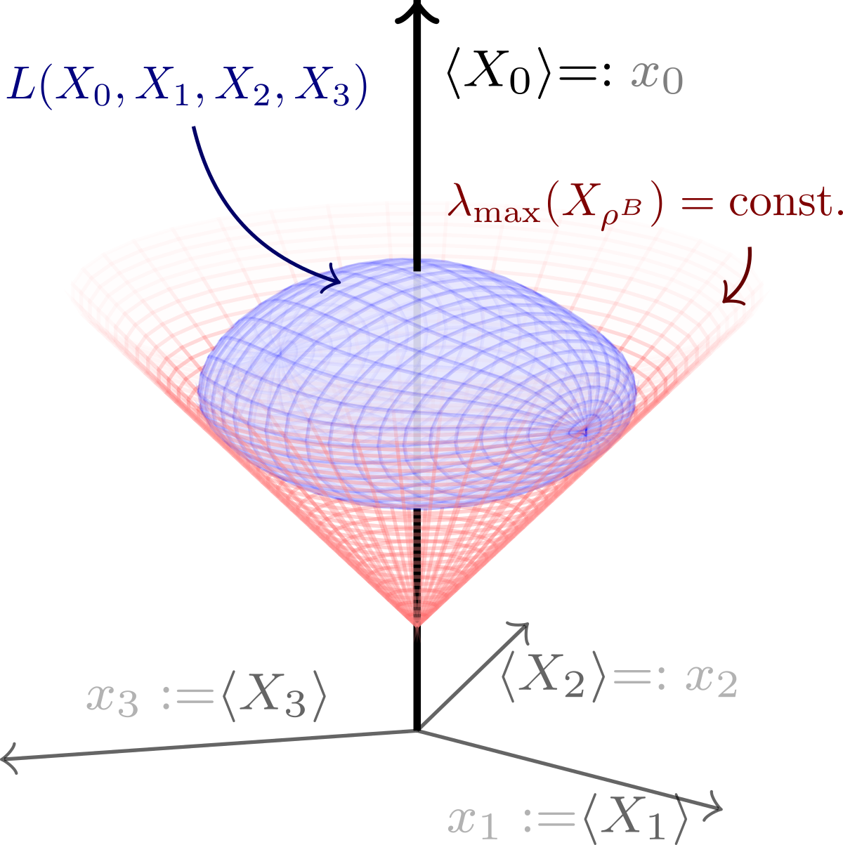
Now the trick is that the isosurface of (2) in the space of $L(X_0, X_1, X_2, X_3)$ can be described by a qudratic polynomial $(x_0-2t)^2-x_1^2-x_2^2-x_3^2$. Furthermore, at least for qubit-qubit systems, the analogue of Kippenhahn theorem works for the task of defining the boundary of $L(X_0, X_1, X_2, X_3)$ in polynomial terms.
The algorithm for finding the analytical description maximal separable expectation value of two-qubit operator $X$ is now as follows.
- Calculate the four matrices $(X_0, X_1, X_2, X_3)$.
- Determine the polynomial description of $L(X_0, X_1, X_2, X_3)$ through the same method as outlined in the Kippenhahn theorem. Generically, the Gröbner basis will contain a linear polynomial (since $L$ is a 3D set embedded in 4D – it is flat!) $l$ and quadratic polynomial $q$ separately.
- Constrain $(x_0-2t)^2-x_1^2-x_2^2-x_3^2$ to the surface defined by the linear equation $l=0$.
- Find the tangent points of the isosurface defined in point 3 with the variety $q=0$.
Example
Consider the operator written in the computational basis of two qubits, $(\ket{00}, \ket{01}, \ket{10}, \ket{11})$:
The relevant matrices are:
The two polynomial equations define the joint numerical range $L(X_0, X_1, X_2, X_3)$:
Now we wish to find the tangent point of the variety defined by the above polynomial equations with the cone $(x_0-2t)^2-x_1^2-x_2^2-x_3^2=0$. First, we remove the $x_3$ variable using the constraint that $l=0$, leading to the constrained equation
Now, in the space of variables $(x_0, x_1, x_2)$ the conditions for tangency are simple: at the point we are looking for, we demand that $q=c=0$ and the normal vectors are collinear, leading to the following final set of polynomial equations
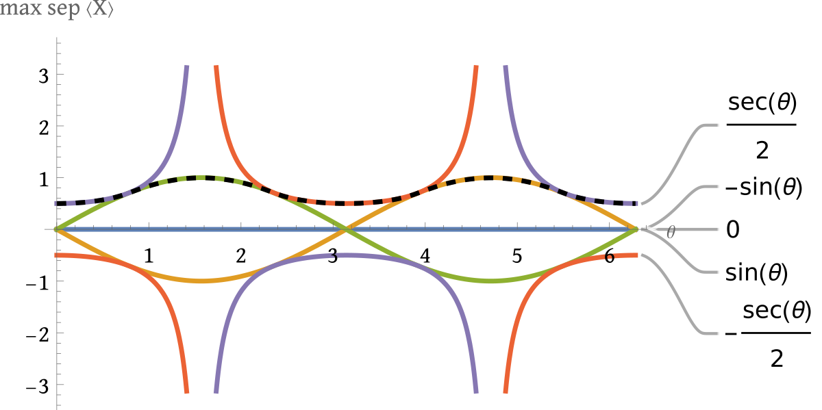
By the usage of standard Gröbner bases algorithms the variables $x_0, x_1, x_2$ are removed, and only a polynomial in $t$ remains. This is the result we are looking for: its roots have the potential to be equal to maximal separable expectation value:
The roots are $t_*=(0,\pm \sin \theta, \pm \frac12 \sec\theta)$. As evidenced by the numerical maximization results (dashed lined in the figure below), the roots indeed correspond to maximal separable expectation values – although it is unclear how to exactly choose the right one: