Quantum Information Geometry

Konrad Szymański

RCQI Bratislava

Quantum mechanics primer

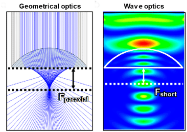
Lee, G. J. et al., Micromachines 2020.

Einstein: light is photons — 'wave components', each with definite energy and wavelength.
de Broglie: … maybe electrons are similar? (yes!)
Schrödinger: insight from the limit
wave optics $\rightarrow$ ray optics, `electron wave' described by $\ket{\psi(t)}=\psi(x,y,z,t)$, \[i \frac{\partial \ket{\psi}}{\partial t} \!=\! \overbrace{\left(\!-(\partial^2_x\!+\!\partial^2_y\!+\!\partial^2_z)\!+\!\frac{k}{\sqrt{x^2\!+\!y^2\!+\!z^2}}\!\right)}^{\hat H} \ket{\psi}\]
Quantum information: restricted linear subspaces of $\ket{\psi}$:\[\ket{\psi} = c_1 \ket{\psi_1} +\ldots+c_d \ket{\psi_d}.\]

What is measurement?

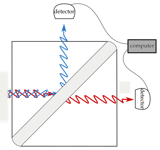
\[\ket{\psi} = {\corange c_1} {\cred \ket{\psi_1}} +\ldots+{\corange c_d} {\cblue \ket{\psi_d}}\cgray = \begin{pmatrix}c_1\\\vdots\\c_d\end{pmatrix}\in\mathbb{C}^d.\]

Separate the parts $\cred \ket{\psi_1}\cblack, \ldots, \cblue\ket{\psi_d}$ in space: clear interpretation!
Born interpretation: probability $\propto~$norm$^2=\lvert {\corange c_k}\rvert^2$ .
We don't know the details!

What is measurement?

From experiment: frequencies of measurement, $P_k\approx\frac{n_k}{\sum_j n_j}$, from Born rule $P_k= \lvert c_k \rvert^2 \cgray = \lvert \langle \psi \vert \psi_k\rangle \rvert^2.$
$P_k$ corresponds to a number $\lambda_k$: weighted average of numbers, expectation value \[\langle \hat A \rangle = \sum \lambda_k P_k.\]
e.g. $\vec\lambda=(-1,0,1)$, $\vec P=(\frac12,0,\frac12) \implies \langle \hat A\rangle=0$
With $\hat A=\sum \lambda_k \ket{\psi_k}\bra{\psi_k},$ ($\hat A$ Hermitian, real eigenvalues) \[\langle \hat A\rangle = \braket{\psi\vert \hat A\vert\psi} \color{gray}= \sum_{i,j=1}^d \psi_i^* A_{i,j} \psi_j.\]

State vectors are not the entire story…

…when information is incomplete.

What if the black box generates $\ket{\psi_k}$ according to the ensemble $\{(p_k,\ket{\psi_k})\}$?

Qubit example:

$$ \hat X = \begin{pmatrix} 0 & 1 \\ 1&0 \end{pmatrix},~ \hat Y = \begin{pmatrix} 0 & -i \\ i & 0 \end{pmatrix}, ~\hat Z=\begin{pmatrix} 1 & 0 \\ 0&-1\end{pmatrix}.$$

With $\ket\psi = \begin{pmatrix} \cos\frac\theta2\\e^{i\phi} \sin\frac\theta2\end{pmatrix},$ $$ \vec r=\begin{pmatrix} \langle \hat X\rangle\\\langle \hat Y\rangle\\\langle \hat Z\rangle\end{pmatrix}=\begin{pmatrix}\cos\phi\sin\theta\\\sin\phi\sin\theta\\\cos\theta\end{pmatrix}, \Vert \vec r \Vert =1 $$ Example for $\cred\ket{0}=\begin{pmatrix}1\\0\end{pmatrix}\cblack, \cblue\ket{1}=\begin{pmatrix}0\\1\end{pmatrix}$: \[\cred\begin{pmatrix} \langle \hat X\rangle\\\langle \hat Y\rangle\\\langle \hat Z\rangle\end{pmatrix}_{\ket0} = \begin{pmatrix}0\\0\\1\end{pmatrix}\cblack,~\cblue\begin{pmatrix} \langle \hat X\rangle\\\langle \hat Y\rangle\\\langle \hat Z\rangle\end{pmatrix}_{\ket1} = \begin{pmatrix}0\\0\\-1\end{pmatrix}\]

If $\cred\ket0\cblack, \cblue\ket1$ are taken at random, \[\langle \hat X\rangle_{\text{ensemble}} =\langle \hat Y\rangle_{\text{ensemble}}= 0,\] \[\langle \hat Z\rangle_{\text{ensemble}} = {\cred \underbrace{\frac12}_{p_{\ket0}} \underbrace{\langle \hat Z\rangle_{\ket0}}_{+1}} + {\cblue \underbrace{\frac12}_{p_{\ket1}} \underbrace{\langle \hat Z\rangle_{\ket1}}_{-1}} \cblack=0 \] \[\lVert \vec r_{\text{ensemble}}\rVert =0!\]

Mixed states are statistical averages

Expectation value linear: \[\sum p_k \braket{\psi_k \vert \hat A\vert \psi_k}=\operatorname{Tr} \hat A \overbrace{\sum p_k \ket{\psi_k} \bra{\psi_k}}^{\hat \rho}\]
$\Tr \begin{pmatrix} X_{1,1}&\ldots&X_{1,d}\\\vdots&\ddots&\vdots\\X_{d,1}&\ldots&X_{d,d}\end{pmatrix}=X_{1,1}+\ldots+X_{d,d}, \Tr(\hat A\cdot \hat B\cdot \hat C)=\Tr(\hat C\cdot \hat A\cdot \hat B)$
Qudit mixed states: \[\mathcal{M_d} = \{ \hat \rho \in \mathbb{C}^{d\times d} : \hat \rho=\hat \rho^\dagger, \operatorname{Tr} \hat \rho=1, \hat \rho \succeq 0\}.\]
$\hat X\succeq 0 \Leftrightarrow \hat X=\sum x_k \ket{\psi_k}\bra{\psi_k}$ with positive $x_k$.
Natural state mixing $p \hat \rho+(1-p) \hat \rho'$, all properties defined by $\hat \rho$. Ensemble details irrelevant.

$\mathcal{M}_2$: the Bloch ball represented by allowed $(\langle \hat X\rangle, \langle \hat Y\rangle, \langle \hat Z\rangle)$.
$\mathcal{M}_3, \mathcal{M}_4$ more complex…

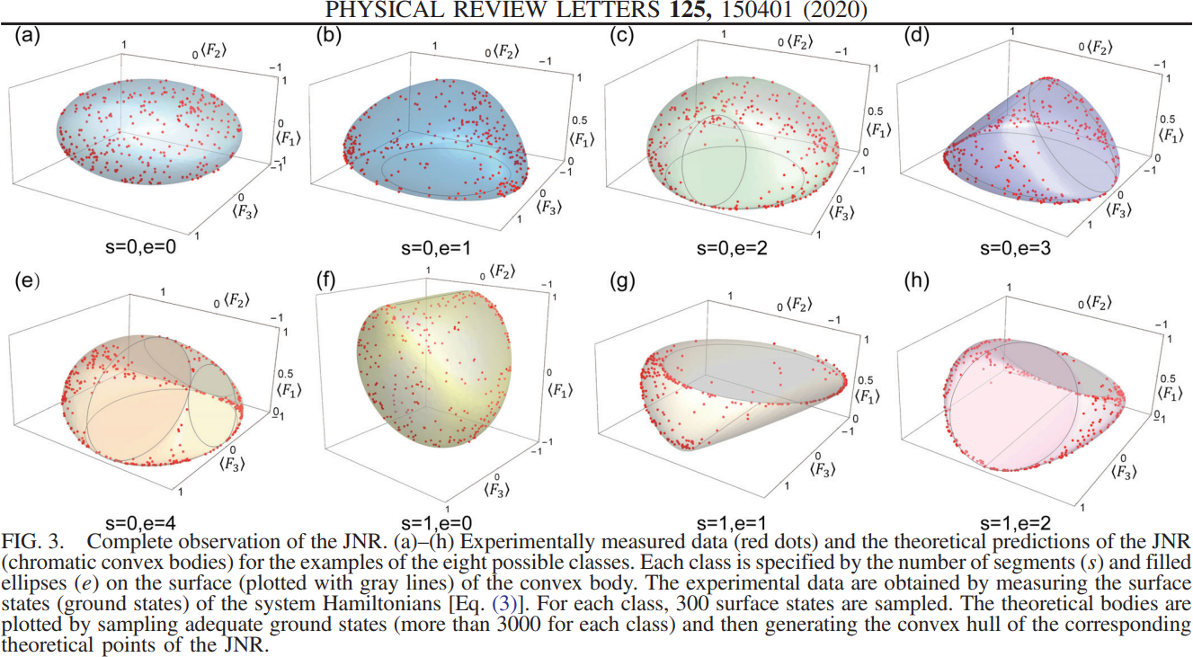
Numerical ranges: projections of state space

(like a photo is a 2D projection of 3D space)

Numerical range: \[W(\hat A_1, \ldots, \hat A_n) \\= \{ (\langle \hat A_1\rangle_{\hat \rho} ,\ldots, \langle \hat A_n \rangle_{\hat \rho}) : \hat \rho \in \mathcal{M} \}\]

$\hat A_i$ Hermitian: \[\langle \hat A\rangle_{\hat \rho} = \Tr \hat A \hat \rho,\] with $\hat A=\sum_{k=1}^d \lambda_k \ket{\psi_k} \bra{\psi_k}.$

$W(X)$: all possible expectation values

$$W(\hat X)=[\lambda_{\min}(\hat X),\lambda_{\max}(\hat X)]$$

$W(\hat X_1, \hat X_2)$: all possible tuples of expectation values

$W(\hat X_1, \hat X_2, \hat X_3)$: triples

J. Xie et al., Observing geometry of quantum states in a three-level system, PRL 2020.

Numerical ranges geometry is defined by polynomials

$$W(\hat X)=[\lambda_{\min}(\hat X),\lambda_{\max}(\hat X)],\color{gray}~~\max(W(\hat X))= \lambda_{\max}(\hat X)$$

$\sim$ max. root of characteristic polynomial $\det(\hat X-\lambda \hat \I)$

$$\max_{(x_1, x_2)\in W(\hat X_1, \hat X_2)} (n_1 x_1+n_2 x_2) = \lambda_{\max} (n_1 \hat X_1+n_2 \hat X_2)$$

$\sim$ max. root of characteristic polynomial $\det(n_1 \hat X_1+n_2 \hat X_2-\lambda \hat \I)$

Polynomial theory!

Uncertainty relations

Variance: from observation statistics (outcome $\lambda_k$ of $\hat A$ with probability $P_k$), \[\operatorname{Var}(\hat A)=\langle (\hat A-\langle \hat A\rangle)^2\rangle=\braket{ \hat A^2}-(\braket{\hat A})^2.\]
Given two measurements $\hat A$ and $\hat B$, what is the relation between variances?
The Heisenberg uncertainty relation: \[\operatorname{Var}({\cred\hat x}) \operatorname{Var}({\cblue\hat p}) \ge \frac{\hbar^2}4,\text{~~for~~}({\cred\hat x} {\psi})\cblack(x)=\cred x\cblack\cdot {\psi}(x)\cblack, ({\cblue\hat p} {\psi})(x) = \cblue-i\hbar\left.\frac{\partial}{\partial x}\cblack{\psi}\right|_{x}\]

Sum of variances: 3D joint numerical range

Goal: Precise magnetic field $B$ measurement ($SU(2)$ metrology)

(Magnetic field changes atoms' properties $\hat X$ and $\hat Y.$ They are measured, and $B$ is reconstructed)

Precision of $B$ bound by variances, $$ \Delta^2(B) \le \text{const.}\times({\operatorname{Var}(\hat X) +\operatorname{Var}(\hat Y)}),$$ for specific $\hat X$ and $\hat Y$.

Goal: find minimal sum of variances \[(x,y,z) \in \cred W(\hat X,\hat Y,\hat X^2+\hat Y^2) \cblack \implies\] \[\cblue \operatorname{Var}(\hat X)+\operatorname{Var}(\hat Y)=z-x^2-y^2.\]

Observation: minimal sum on variances on the surface of $\cred W(\hat X,\hat Y,\hat X^2+\hat Y^2)$.
Tangent to the paraboloid.

Goal: find tangent paraboloid. With \[f(x,y,\lambda):=\det((\hat X-x \hat \I)^2+(\hat Y-y\hat \I)^2-\lambda \I),\] tangent points defined by \[f=0,~\frac{\partial f}{\partial x}=0,\frac{\partial f}{\partial y}=0.\]

Result: polynomial in $\lambda$, minimal root$\sim$minimal sum of variances.

Summary

Different definition of sets of quantum states help in some cases.
Numerical ranges (possible tuples of expectation values) are their projections, with polynomial theory connection.
Uncertainty relations for accurate measurements can be determined this way.

Thank you for your attention!

References:

K.S., Numerical ranges and geometry in quantum information: Entanglement, uncertainty relations, phase transitions, and state interconversion (PhD thesis), arXiv: 2303.07390,
K.S., S. Weis, K. Życzkowski, Classification of joint numerical ranges of three hermitian matrices of size three, LAA 2018,
T. Simnacher, J. Czartowski, K.S., K. Życzkowski, Confident entanglement detection via the separable numerical range, PRA 2021,
K.S., K. Życzkowski, Geometric and algebraic origins of additive uncertainty relations, J Phys A 2019,
Lee, G. J. et al., Micromachines 2020.
J. Xie et al., PRL 2020

Correlation between different parts of the system

State of two systems: $\rho\in \mathcal{M}_{d_1\times d_2}$
($\rho=$ convex combination of projectors onto subspaces in $\mathcal{H}_{d_1}\otimes\mathcal{H}_{d_2} $)
No correlation at all: $\rho = \rho' \otimes \rho''$
Any non-tensor $\rho$: correlation when measuring two subsystems!
Definition (separable states of bipartite $\mathcal{H}_{d_1}\otimes\mathcal{H}_{d_2}$): \[ \mathcal{M}^{\text{sep}}_{d_1,d_2} = \operatorname{conv}\{ \Pi_{\ket{v_k'}}\otimes \Pi_{\ket{v_k''}}: \ket{v'}\in\mathcal{H}_{d_1}, \ket{v''}\in\mathcal{H}_{d_2}\} \]
$\mathcal{M}^{\text{sep}}_{d_1,d_2}$ allows for correlations… but not all of them!

$\mathcal{M}^{\text{sep}}_{d_1,d_2}$ is a proper convex subset of $\mathcal{M}_{d_1\times d_2}$.

Entanglement and separable numerical ranges

Joint numerical range vs separable numerical range

$W_{\text{sep}}=\{\vec a \in \mathbb{R}^n | a_i = \operatorname{Tr} \rho A_i, \rho \in \mathcal{M}^{\text{sep}}\}$
Expectation values outside $W_{\text{sep}}~\implies$ entanglement!
$W_{\text{sep}}$ convex $\implies$ defined by linear constraints.
Approximation by half-space intersection in general NP-hard!
S. Friedland, L-H. Lim, Nuclear Norm of Higher-Order Tensors, Math. Comp. 2014

Entanglement and separable numerical ranges

Goal: maximize $\operatorname{Tr} X(\rho'\otimes \rho'')$ over $ \rho'\in\mathcal{M}_2, \rho''\in\mathcal{M}_d $.

Lemma: Optimization reduces to finding a point on the surface of 4D joint numerical range, tangent to a hypercone.

Main points:

$ \operatorname{Tr} X (\rho'\otimes \rho'')=\operatorname{Tr} \rho' X''$, where \[X''=\operatorname{Tr}_2 X (\operatorname{Id} \otimes \rho'')\]
For $\rho''$ fixed, \[\max_{\rho'} \operatorname{Tr} \rho' X'' = \lambda_{\max}(X'').\]
$X'' \in M_{2\times 2} \implies $ for $X_i=\operatorname{Tr}_1 X(\sigma_i\otimes \operatorname{Id})$, \[\lambda_{\max}(X'')=x_0+\sqrt{x_1^2+x_2^2+x_3^2}\]
Linearization possible: then semidefinite programming.

$\operatorname{Tr}_2$: linear extension of \[\operatorname{Tr}_2 A \otimes B = A \operatorname{Tr} B.\] Similarly, \[\operatorname{Tr}_1 A \otimes B=B \operatorname{Tr} A.\]